Multi-Frequency Matter Profiles
The approach applied to the neutrino flavor transformation with a single-frequency matter profile can also be used in more general cases with multi-frequency matter profiles. Even though there is only one Rabi mode that is on resonance, the presence of many off-resonance Rabi modes may interfere with the on-resonance mode and suppress or enhance the neutrino flavor conversions.
I will consider a matter profile with two Fourier modes: $$ \begin{equation} \lambda(r) = \lambda_0 + \lambda_1 \cos (k_1 r) + \lambda_2 \cos (k_2 r). \end{equation} $$ The Hamiltonian for the neutrino oscillations in the background matter basis is $$ \begin{align} \mathsf H^{(\mm)} =& - \frac{\omega_\mm}{2}\sigma_3 + \frac{1}{2} \left( \lambda_1 \cos(k_1 r) + \lambda_2 \cos(k_2 r) \right) \cos 2\theta_\mm \sigma_3 \nonumber\\ &- \frac{1}{2} \left( \lambda_1 \cos(k_1 r) + \lambda_2 \cos(k_2 r)\right)\sin 2\theta_\mm \sigma_1. \label{eq-hamiltonian-bg-matter-basis-multi-frequency} \end{align} $$ I will drop the oscillating $\sigma_3$ terms for the same reason as in the single-frequency matter profile case. The Hamiltonian becomes $$ \begin{equation} \mathsf H^{(\mm)} \to - \frac{\omega_\mm}{2}\sigma_3 - \sum_{n}\frac{A_n}{2} \cos(k_n r) \sigma_1 + \sum_n\frac{A_n}{2} \sin(k_n r) \sigma_2. \label{eq-hamiltonian-bg-matter-basis-multi-frequency-drop-varying-sigma3} \end{equation} $$ There are four Rabi modes in this Hamiltonian, $n=1+$, $1-$, $2+$, and $2-$. The amplitudes and wavenumbers of the four Rabi modes are $$ \begin{align} A_{1\pm} &= \frac{\lambda_1 \sin (2\theta_\mm)}{2}, & k_{1\pm} &= \pm k_1, \\ A_{2\pm} &= \frac{\lambda_2 \sin (2\theta_\mm)}{2}, & k_{2\pm} &= \pm k_2, \end{align} $$ respectively.
Transition Probabilities with Reduction
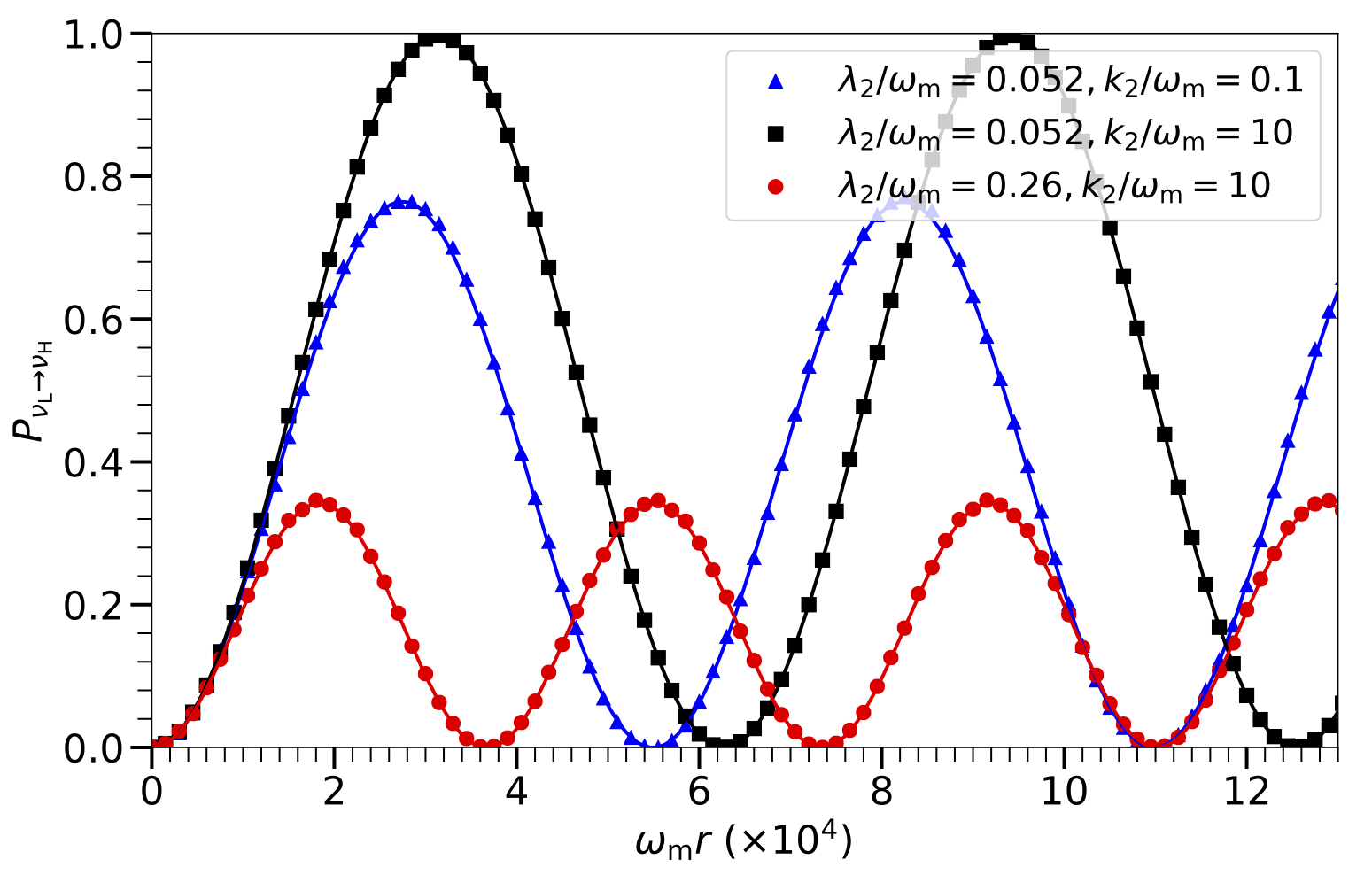
The transition probabilities as functions of distance $r$ for a neutrino propagating through matter profile of the form $\lambda(r) = \lambda_0 + \lambda_1 \cos (k_1 r) + \lambda_2 \cos (k_2 r)$ with different values of $\lambda _ 2$ and $k _ 2$ as labeled. The markers are for the numerical results obtained by using the Hamiltonian in Eqn. \eqref{eq-hamiltonian-bg-matter-basis-multi-frequency}, and the continuous curves are obtained using the Rabi formula in Eqn. \eqref{app:rabi-system-transition-probability} but with the values of the modified relative detunings $\RD' _ {2+}$ in Table multi-frequency-rabi-simple-relative-detuning-destruction. In all three cases, $\lambda_0$ is half of the MSW resonance potential, $\lambda_1/\omega_\mm = 5.2\times 10^{-4}$ and $k_1/\omega_\mm = 1$.
| $\lambda_2/\omega_\mm$ | $k_2/\omega_\mm$ | $D'_ {(1-)}$ | $D' _ {(2+)}$ | $D'_ {(2-)}$ |
|---|---|---|---|---|
| $0.052$ | $0.1$ | $2.5\times 10^{-5}$ | 0.56 | 0.46 |
| $0.052$ | $10$ | $2.5\times 10^{-5}$ | 0.056 | 0.045 |
| $0.26$ | $10$ | $2.5\times 10^{-5}$ | 1.4 | 1.1 |
The above Table multi-frequency-rabi-simple-relative-detuning-destruction shows the relative detunings of the Rabi resonance when only the $1+$ mode and another Rabi mode are considered.
The presence of the additional Fourier mode can suppress the Rabi resonance. This is illustrated in Fig. Transition Probabilities with Reduction. In this figure, I choose the $1+$ Rabi mode to be exactly on resonance with $\lambda_1/\omega_\mm=5.2\times 10^{-4}$ and $k_1/\omega_\mm=1$. The triangles represent the numerical solution for neutrino flavor transformation with $\lambda_2/\omega_\mm=0.052$ and $k_2/\omega_\mm=0.1$. One can see that the transition amplitude is suppressed due to the presence of the second Fourier mode. I used Eqn.~\eqref{app:chap:matter-eq:relative-detuning-changed} to calculate the modified relative detunings by taking into account only the $1+$ mode and another Rabi mode. The values of the relative detunings are listed in Table table:multi-frequency-rabi-simple-relative-detuning-destruction. I calculated the transition probability using the Rabi formula in Eqn.~\eqref{app:rabi-system-transition-probability} with the relative detuning $\RD'_{(2+)}$ (the continuous curve in the figure), and it agrees with the numerical solution very well. I also showed two additional examples with $(\lambda_2/\omega_\mm, k_2/\omega_\mm)$ being $(0.052, 10)$ and $(0.26, 10)$, respectively. In both examples, the numerical solutions and the analytic results by using the Rabi formula have excellent agreement.
Transition Probabilities with Enhancement
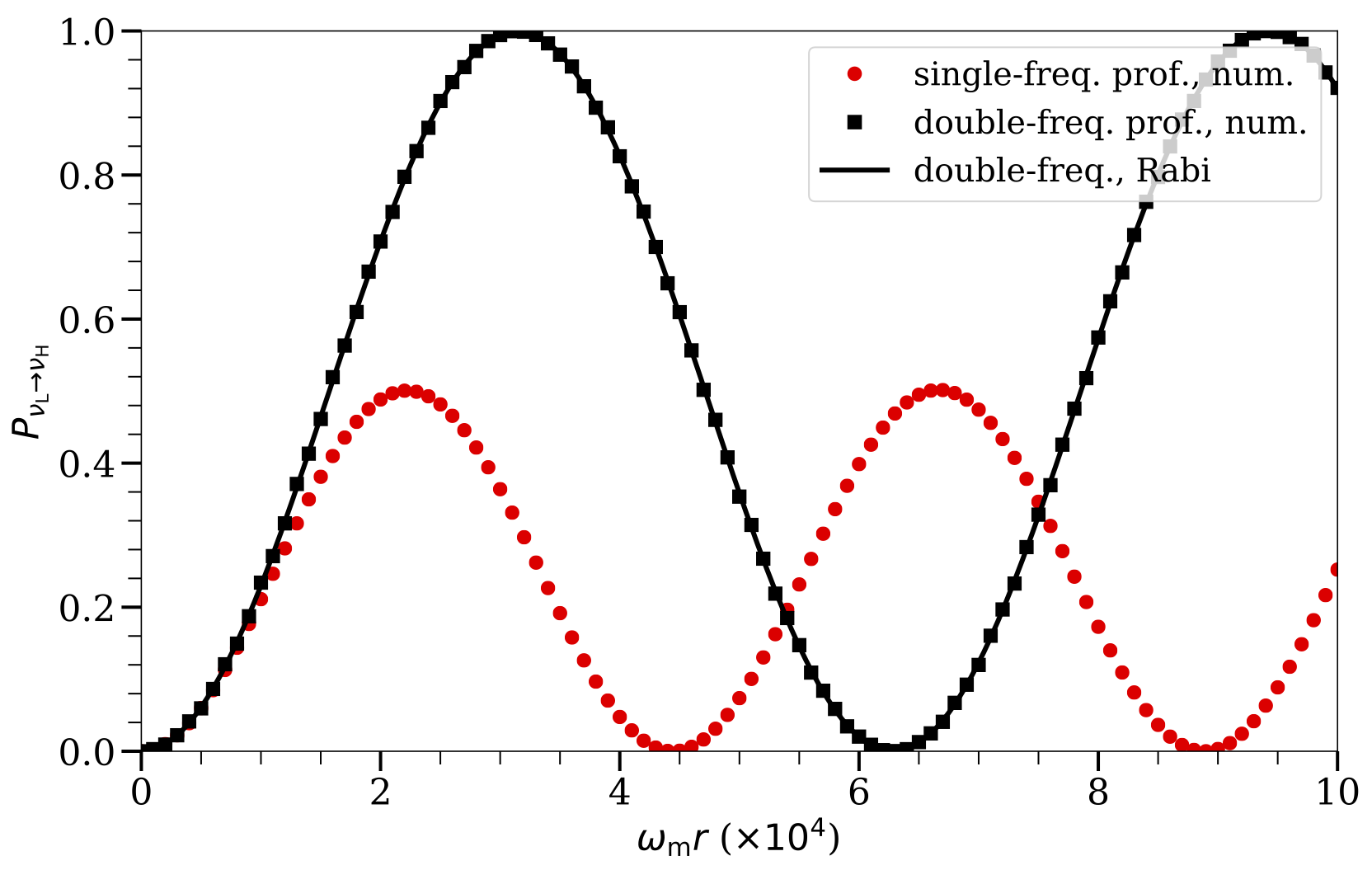
The presence of the second Fourier mode can also enhance the Rabi resonance, which is illustrated in Fig. Transition Probabilities with Enhancement. The two Fourier modes in this figure have amplitudes and wavenumbers $$ \begin{align*} \lambda_1/\omega_\mm & =5.2\times 10^{-4}, & k_1/\omega_\mm &= 1- 10^{-4},\\ \lambda_2/\omega_\mm & =0.1, & k_2/\omega_\mm &= 3, \end{align*} $$ respectively. The neutrino flavor conversion is never complete if only the first Fourier mode is present because the relative detuning $\RD_{1+}=1 > 0$. This is shown as the red dots in the figure. However, complete neutrino flavor conversion occurs when both Fourier modes are present. This is because the modified relative detuning $\RD'_{(2+)} = 0$ when only the $1+$ and the $2+$ Rabi modes are considered. The numerical solution and the analytic prediction using the Rabi formula are plotted as the black squares and the continuous curve, respectively, which agree very well.