Vacuum Oscillations
Neutrino vacuum oscillations
Before carrying out the calculations, I can estimate the frequency of the oscillations of the neutrino between its flavors. In natural units, frequency has the same dimension as energy.
Consider an electron neutrino with momentum $p$ which is a superposition of the two mass eigenstates $\ket{\nu_i}$ ($i=1,2$) with masses $m_i$, respectively. Since the neutrino masses are small, I can Taylor expand the energy of each mass eigenstate in terms of the corresponding mass:
$$ \begin{align} E_i & = \sqrt{m_i^2 + p^2 } \nonumber\\ & = p \sqrt{\frac{m_i^2}{p^2} + 1} \nonumber\\ & \approx p + \frac{1}{2} \frac{m_i^2}{p}. \label{chap:basics-section:neutrinos-eqn:energy-taylor} \end{align} $$The first term in the above equation produces a global phase to the flavor wave function of the neutrino which does not affect neutrino flavor oscillations. The characteristic energy scale in the problem is the difference between the energies of the two mass eigenstates, $$ \begin{equation} \omega_{\mathrm v} = E_2-E_1 = \frac{m_2^2-m_1^2}{2E} = \frac{\delta m^2}{2E}, \label{chap:basics-section:neutrinos-eqn:qualitative-method-frequency} \end{equation} $$ which turns out to be the vacuum oscillation frequency. Here $E=p$ is approximately the energy of the neutrino.
To work out the exact solution, I will utilize the Schrödinger equation. First of all, the flavor eigenstates are denoted as $\ket{\nu_\alpha}$ where ${}_\alpha$ can be ${}_{\mathrm{e}}$ or ${}_{\mathrm{x}}$ for the electron flavor and the other flavor. The wave function of the neutrino state $\ket{\nu}$ in the flavor basis, defined as
$$ \Psi^{(\ff)} = \begin{pmatrix} \psi^{(\ff)}_{\mathrm e} \\\\ \psi^{(\ff)}_{\mathrm x} \end{pmatrix} = \begin{pmatrix} \braket{\nu_{\mathrm e}}{\nu} \\\\ \braket{\nu_{\mathrm x}}{\nu} \end{pmatrix}, $$is related to the wave function in the vacuum mass basis $\Psi^{(\vv)}$ through a unitary mixing matrix $\mathsf U$,
$$ \begin{equation} \Psi^{(\mathrm f)} = \mathsf{U}\Psi^{(\vv)}, \label{chap:vacuum-eqn:wavefunction} \end{equation} $$where the upper indices ${}^{(\vv)}$ and ${}^{(\ff)}$ are used to denote the corresponding bases. The mixing matrix can be expressed using the vacuum mixing angle $\theta_{\vv}$: $$ \mathsf{U} = \begin{pmatrix} \cos\theta_\vv & \sin \theta_\vv \\ -\sin \theta_\vv & \cos \theta_\vv \end{pmatrix}. $$ In the vacuum mass basis, the neutrino has a free propagation Hamiltonian $$ \mathsf H^{(\vv)} = \begin{pmatrix} E_1 & 0 \\ 0 & E_2 \end{pmatrix}. $$ To the first order, the Hamiltonian becomes $$ \begin{align} \mathsf H^{(\vv)} &\approx \frac{1}{2E} \begin{pmatrix} m_1^2 & 0 \\ 0 & m_2^2 \end{pmatrix} + E \mathsf{I} \nonumber \\ & = \frac{1}{4E} \begin{pmatrix} - \delta m^2 & 0 \\ 0 & \delta m^2 \end{pmatrix} + \left(\frac{m_2^2 + m_1^2}{4E} + E \right) \mathsf{I}. \end{align} $$ Because a multiple of the identity matrix $\mathsf{I}$ gives only a global phase to the neutrino flavor wave function, I will neglect it from now on, and the vacuum Hamiltonian simplifies to $$ \begin{equation} \mathsf H^{(\vv)} \to \frac{\delta m^2}{4E} \begin{pmatrix} -1 & 0 \\ 0 & 1 \end{pmatrix} = -\frac{\delta m^2}{4E} \sigma_3 = -\frac{\omega_{\vv}}{2}\sigma_3, \end{equation} $$ where $$ \begin{align} \sigma_1 &= \begin{pmatrix} 0 & 1 \\ 1 & 0 \end{pmatrix}, &\sigma_2 &= \begin{pmatrix} 0 & -\ii \\ \ii & 0 \end{pmatrix}, &\sigma_3 &= \begin{pmatrix} 1 & 0 \\ 0 & -1 \end{pmatrix} \end{align} $$ are the three Pauli matrices. The Schrödinger equation has the following simple solution in the mass basis: $$ \begin{equation} \Psi^{(\vv)}(t) = \begin{pmatrix} c_1(0) e^{i \omega_\vv t/2 } \\ c_2(0) e^{ -i\omega_\vv t/2 } \end{pmatrix}. \end{equation} $$
Using Eqn. \eqref{chap:vacuum-eqn:wavefunction}, I obtain the wave function in the flavor basis, $$ \begin{align} \Psi^{(\ff)}(t) &= \mathsf{U}\Psi^{(\vv)}(t) \\ & = \begin{pmatrix} \cos\theta_\vv & \sin \theta_\vv \\ -\sin \theta_\vv & \cos \theta_\vv \end{pmatrix} \begin{pmatrix} c_1(0) e^{i\omega_\vv t/2 } \\ c_2(0) e^{ -i\omega_\vv t/2 } \end{pmatrix} . \label{chap:vacuum-eqn:wavefuncion-time} \end{align} $$ Alternatively, I can also determine the Hamiltonian in the flavor basis first, which is $$ \begin{equation} \mathsf H^{(\ff)} = \mathsf U \mathsf H^{(\vv)} \mathsf U^\dagger = -\frac{\omega_\vv}{2}\cos 2\theta_\vv \sigma_3 + \frac{\omega_\vv}{2} \sin 2\theta_\vv \sigma_1. \label{chap:basics-sec:vacuum-osc-eqn:hamiltonian-vacuum} \end{equation} $$ By solving the Schrödinger equation in the flavor basis, I will obtain the same wave function as in Eqn. \eqref{chap:vacuum-eqn:wavefuncion-time}.
The probability for a neutrino emitted in the electron flavor at time $t=0$ to be detected as the electron flavor at a later time $t$ is \begin{equation} P(t) = 1-\sin^2(2\theta_\vv)\sin^2\left( \frac{\omega_\vv t}{2} \right). \end{equation} Since the neutrino travels with approximately the speed of light, the electron neutrino survival probability at a distance $r$ from the source is $$ \begin{equation} P(r) = 1-\sin^2(2\theta_\vv)\sin^2\left( \frac{\omega_\vv}{2} r \right). \label{chap:basics-eqn:vacuum-electron-probability} \end{equation} $$ I plot the above result in the following figure which clearly shows the oscillatory behavior. The oscillation length is determined by the characteristic energy scale $\omega_\vv$, which confirms our estimation in Eqn. \eqref{chap:basics-section:neutrinos-eqn:qualitative-method-frequency}. The oscillation amplitude is determined by $\sin^2(2\theta_\vv)$.
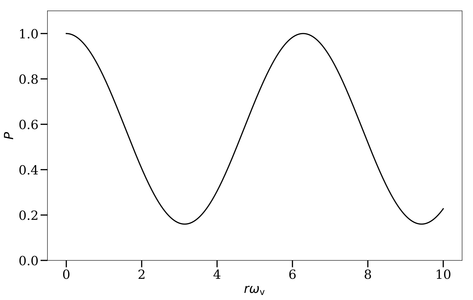
Two-Flavor Oscillations in Vacuum
The electron flavor neutrino survival probability in vacuum oscillations as a function of distance $r$ which is measured in terms of vacuum oscillation frequency $\omega_\vv$. The mixing angle $\theta_\vv$ is given by $\sin^2\theta_\vv=0.30 \approx \sin^2 \theta_{12}$.
In nature, there are three neutrino flavors and, correspondingly, three neutrino mass eigenstates as shown in the following figures. The order of the three neutrino masses. The difference between the first two masses is responsible for solar neutrino oscillations, and the difference between the third mass and the first two is responsible for atmospheric neutrino oscillations.
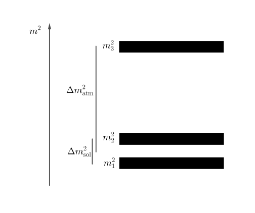
Normal hierarchy: the third mass is larger than the first two.
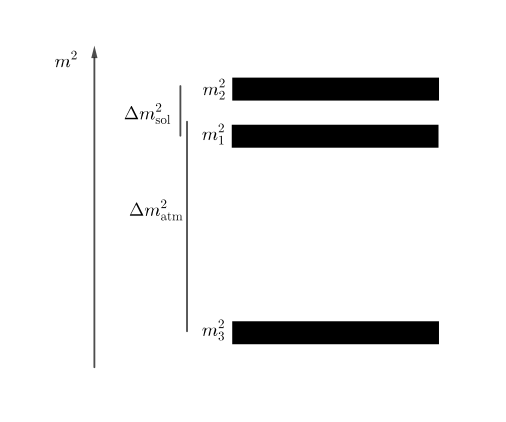
Inverted hierarchy: the third mass is smaller than the first two.
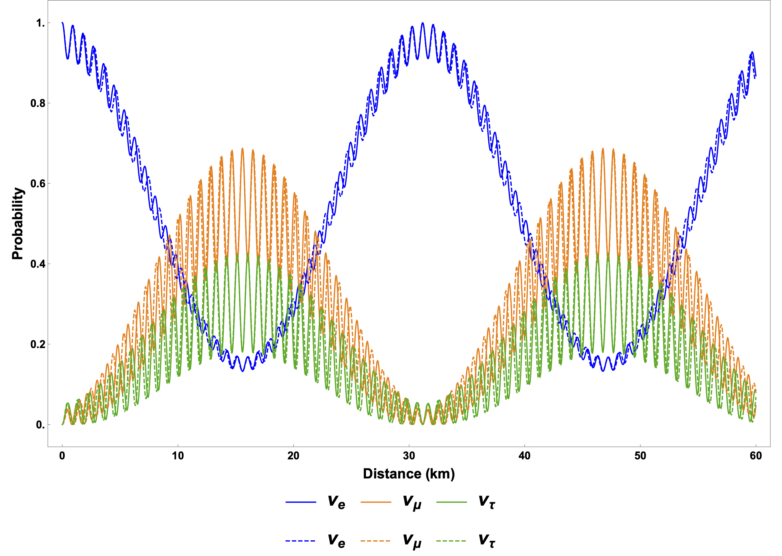
Because there are two different characteristic energy scales, $\omega_{\vv,21}=\delta m_{21}^2/2E$ and $\omega_{\vv,32}=\delta m_{31}^2/2E$, two oscillation periods should occur, as shown in the figure bellow. The fast oscillations are determined by the larger energy scale, $\omega_{\vv,32}$, while the slow oscillations are determined by the smaller one $\omega_{\vv,21}$. For the inverted neutrino mass hierarchy (with $m_3 < m_1 < m_2$), the oscillation frequencies are the same as in the normal mass hierarchy (with $m_3>m_2>m_1$) since they have the same characteristic energy scales. However, they will develop different phases during oscillations.