Single-Frequency Matter Profiles

I will examine the neutrino flavor conversion in a single-frequency matter profile $\delta\lambda(r) = \lambda_1 \cos(k_1 r)$. I will assume that the perturbation is small so that $\lambda_1 \ll \omega_\mm$. The Hamiltonian in the background matter basis becomes $$ \begin{equation} \mathsf H^{(\mm)} = - \frac{\omega_\mm}{2}\sigma_3 + \frac{1}{2} \lambda_1 \cos(k_1 r) \cos 2\theta_\mm \sigma_3 - \frac{1}{2} \lambda_1 \cos(k_1 r)\sin 2\theta_\mm \sigma_1. \label{chap:matter-sec:single-fequency-eq:hamiltonian-bg-matter-basis-single-frequency} \end{equation} $$ I will consider the case when $k_1$ is not far away from resonance, i.e., $k_1 \sim \omega_\mm$. As will be proven later, the oscillating $\sigma_3$ term in the above Hamiltonian has little effect on the transition probabilities in this case. With the oscillating $\sigma_3$ term removed, $$ \begin{align} \mathsf H^{(\mm)} &\to -\frac{\omega_{\mathrm m}}{2} \sigma_3 - \frac{1}{2} A_1 \cos ( k_1 r) \sigma_1 + \frac{1}{2} A_1\sin(k_1 r) \sigma_2 \nonumber\\ &\phantom{\to} - \frac{1}{2} A_2 \cos ( k_2 r) \sigma_1 + \frac{1}{2} A_2\sin(k_2 r) \sigma_2 \label{eq-hamiltonian-bg-matter-basis-single-frequency} \end{align} $$ where $$ \begin{align} A_1 = A_2 = \frac{\lambda_1 \sin(2\theta_\mm) }{2} \quad \text{and} \quad k_2 = -k_1. \label{chap:matter-sec:single-eqn:rabi-amplitudes} \end{align} $$ This is the same as the Hamiltonian $\mathsf H_{\RR}$ in Eqn. \eqref{chap:matter-sec:single-frequency-eqn:hamiltonian-two-level}. Because the second Rabi mode is off resonance and its amplitude is too small to satisfy the criterion in Eqn. \eqref{chap:matter-sec:single-frequency-eqn:criterion-for-a2}, it can be neglected and Rabi formula in Eqn. \eqref{app:rabi-system-transition-probability} can be applied with $A_\RR=A_1$, $k_\RR=k_1$, and $\omega_\RR = \omega_\mm$.

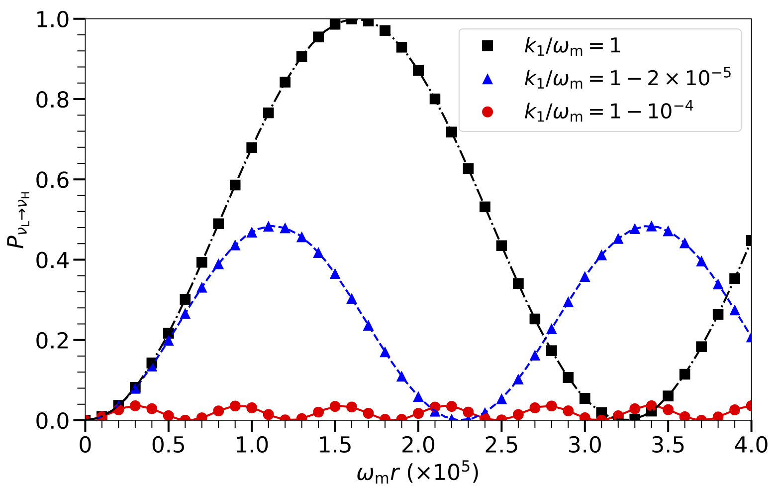
I calculated the transition probability using the Hamiltonian in Eqn. \eqref{chap:matter-sec:single-fequency-eq:hamiltonian-bg-matter-basis-single-frequency} with $k_1/\omega_\mm=1$ and plotted it as black square markers in Fig. Neutrino Rabi Oscillations for Single Mode. For comparison I also plotted the transition probability obtained from the Rabi formula in Eqn. \eqref{app:rabi-system-transition-probability} as the dot-dashed curve in the same figure, which agrees with the numerical result very well. In this case, the first Rabi mode is exactly on resonance with relative detuning $\RD_1=0$. I calculated the transition probabilities for additional two cases with $k_1/\omega_\mathrm{m}=1-2\times 10^{-5}$ and $1-10^{-4}$, which have relative detunings $\RD_1 = 1$ and $5.2$, respectively. The Rabi resonance is suppressed as $\RD_1$ increases. The results obtained using the full Hamiltonian and those from the Rabi formula again agree very well.

The transition probabilities $P_{\nu_\mathrm{L}\to\nu_\mathrm{H}}$ as functions of distance $r$ for a neutrino propagating through matter profiles of the form $\lambda(r)=\lambda_0 + \lambda_1 \cos (k_1 r)$ with different values of $k_1$ as labeled. The markers are for the numerical results obtained by using the Hamiltonian in Eqn. \eqref{chap:matter-sec:single-fequency-eq:hamiltonian-bg-matter-basis-single-frequency}, and the continuous curves are obtained using the Rabi formula in Eqn. \eqref{app:rabi-system-transition-probability}. In all three cases, $\lambda_0$ is half of the MSW resonance potential, and $\lambda_1/\omega_\mm=5.2\times 10^{-4}$.

For a single-frequency perturbation in the matter profile $\lambda(r) =\lambda_0 + \lambda_1\sin(k_1 r)$, P. Krastev and A. Smirnov concluded that the parametric resonance condition is $\omega_{\mathrm{m}} \sim n k_1$ if $$ \begin{equation} \omega_{\mathrm{m,inst}}(r) = \omega_{\mathrm{v}} \sqrt{ \left[ \lambda(r)/\omega_{\mathrm{v}} - \cos (2\theta_{\mathrm{v}}) \right]^2 + \sin^2(2\theta_{\mathrm{v}}) } \end{equation} $$ varies slowly with $r$ ¹. This condition is exactly the Rabi resonance condition when $n=1$. Higher order effects will be explained in Sec. Single-Frequency Matter Profiles Revisted.

Edit this page on GitHub