Rabi Oscillations
Rabi Oscillations
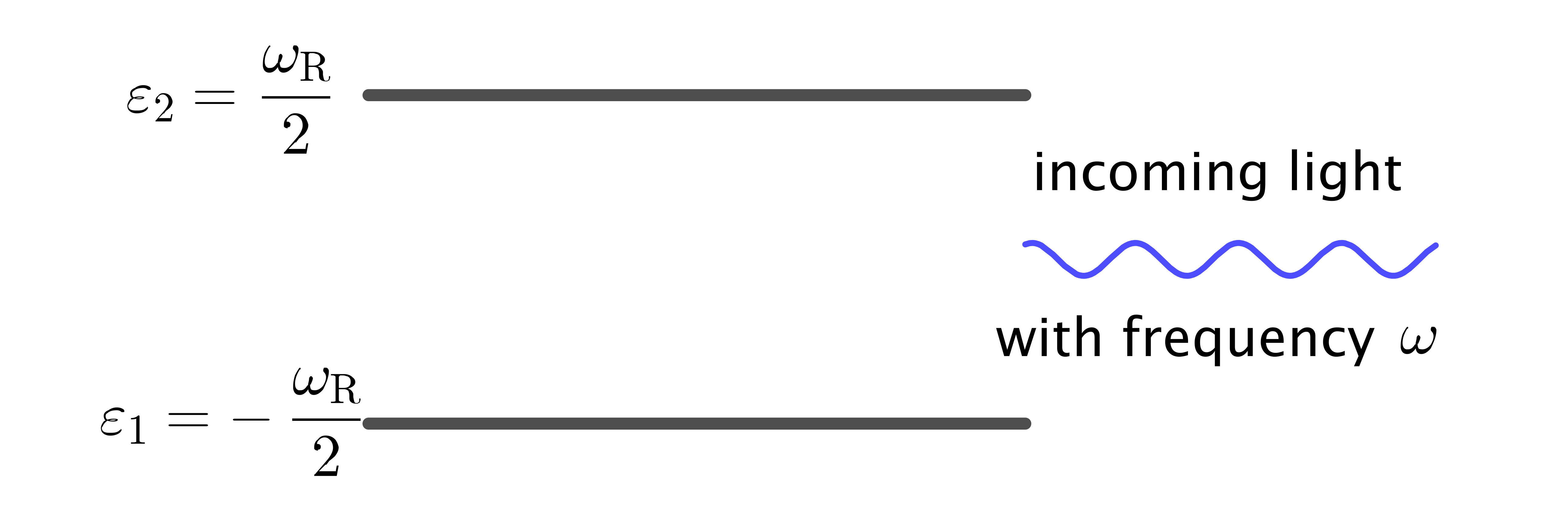
A two-level quantum system that experiences the Rabi oscillations. The resonance occurs when the frequency of the driving field $\omega$ equals the energy gap $\omega_\RR = \varepsilon_2 - \varepsilon_1$.
A two-level quantum system with energy gap $\delta\varepsilon = \omega_{\RR}$ can experience Rabi oscillations when some light with frequency $\omega$ shines on it (see Fig. Rabi Oscillations).
The Hamiltonian for the system is $$ \begin{equation} \mathsf H_{\RR} = -\frac{\omega_{\RR}}{2}\sigma_3 - \frac{A_{\RR} }{2} \left( \cos(k_{\RR} t)\sigma_1 - \sin(k_{\RR} t) \sigma_2\right), \label{rabi-oscillation-single-perturbation} \end{equation} $$ where $A_{\RR}$ and $k_{\mathrm{R}}$ are the amplitude and frequency of the driving field, respectively. The Hamiltonian $\mathsf H_\RR$ can be mapped on to a vector using the flavor isospin picture: $$ \begin{equation} \vec H_{\RR} = \vec H_3 + \vec H_+, \label{chap:matter-eqn:rabi-hamiltonian-h3-hplus} \end{equation} $$ where $$ \begin{equation} \vec{H}_3 = \begin{pmatrix} 0 \\ 0 \\ \omega_{\mathrm R} \end{pmatrix} \quad \text{and} \quad \vec{H}_+ = \begin{pmatrix} A_{\mathrm{R}} \cos(k_{\mathrm{R}} t ) \\ - A_{\mathrm{R}} \sin(k_{\mathrm{R}} t) \\ 0 \end{pmatrix}. \label{chap:app-sec:rabi-eqn:h3-and-hplus} \end{equation} $$ The vector $\vec{H}_3$ is the vector aligned with the third axis and $\vec{H}_+$ is a vector rotating in a plane perpendicular to $\vec{H}_3$ (see Fig. Rabi Frames). The wave function $\Psi=(\psi_1,\psi_2)^{\mathrm{T}}$ is also used to define the state vector $\vec{s}$ $$ \begin{equation} \vec{s} = \Psi^\dagger \frac{\vec{\sigma}}{2}\Psi = \frac{1}{2}\begin{pmatrix} 2\,\mathrm{Re}\,(\psi_1^* \psi_2) \\ 2\,\mathrm{Im}\,(\psi_1^*\psi_2) \\ \lvert \psi_1 \rvert^2 - \lvert \psi_2 \rvert^2 \end{pmatrix}. \end{equation} $$
Rabi Frame
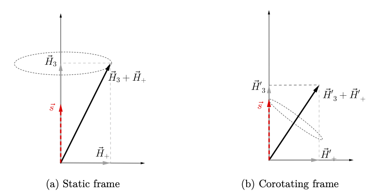
Rabi oscillations in different frames. The vectors $\vec H_3$ and $\vec H_+$ are defined in Eqn. \eqref{chap:app-sec:rabi-eqn:h3-and-hplus}. The red dashed vector $\vec s$ represents the quantum state of the system, and the black solid vectors are for the Hamiltonians in the corresponding frames.
The third component of $\vec{s}$, which is denoted as $s_3$, is within the range $[-1/2,1/2]$. The two limits, $s_3=-1/2$ and $s_3=1/2$ stand for the high energy state and the low energy state of the two-level system, respectively. If the two-level system has equal probabilities to be in the high energy state and the low energy state, one has $s_3=0$. The equation of motion of $\vec s$ is the same as Eqn. \eqref{chap:basics-sec:flavor-isospin-pic-eqn:eom-precession} and describes the precession of $\vec s$.
In this example, the total “Hamiltonian vector” $\vec H_\RR$ is not static since it has a rotating component $\vec H_+$. A more convenient frame is the one that corotates with $\vec{H}_+$, which is depicted in Fig. Rabi Frames. The equation of motion of $\vec s$ in this frame is $$ \begin{equation} \frac{\mathrm d}{\mathrm d t } \vec{s} = \vec{s} \times (\vec{H}'_3 + \vec{H}_+), \end{equation} $$ where $$ \begin{equation} \vec{H}'_3 = \begin{pmatrix} 0 \\ 0 \\ \omega_{\mathrm{R}} - k_{\mathrm R} \end{pmatrix} \quad \text{and} \quad \vec{H}'_+ = \begin{pmatrix} A_{\mathrm{R}} \\ 0 \\ 0 \end{pmatrix}. \end{equation} $$ The state vector $\vec{s}$ precesses around the static vector $\vec{H}'_3 + \vec{H}'_+$ in this corotating frame with a frequency $$ \begin{equation} \Omega_{\mathrm R} = \sqrt{ \lvert A_{\mathrm{R}}\rvert^2 + (k_{\mathrm{R}} - \omega_{\mathrm R})^2 } \label{app:rabi-frequency} \end{equation} $$ which is known as the Rabi frequency. Projecting the state vector $\vec{s}$ on to the third axis, I obtain $$ \begin{equation} s_3 = \frac{1}{2} - \frac{\lvert A_{\mathrm R}\rvert ^2}{\Omega_{\mathrm R}^2}\sin^2\left(\frac{\Omega_{\mathrm R}}{2} t\right). \end{equation} $$ Such a system has a transition probability from the low energy state to the high energy state, given by the Rabi formula, $$ \begin{equation} P(t) = \frac{1}{2}\left[ 1- 2 s_3(t) \right] = \frac{1}{ 1 + \RD^2 } \sin^2 \left( \frac{\Omega_{\mathrm R}}{2} t \right), \label{app:rabi-system-transition-probability} \end{equation} $$ where $$ \begin{equation} \RD = \left\lvert \frac{ k_{\mathrm R} - \omega_{\mathrm R}}{A_{\mathrm R}} \right\rvert. \label{chap:app-sec:rabi-oscillations-eqn:relative-detuning-def} \end{equation} $$ is the relative detuning.
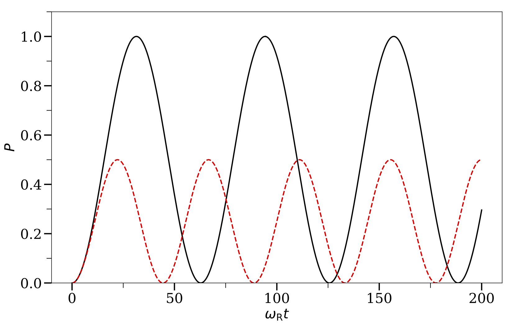
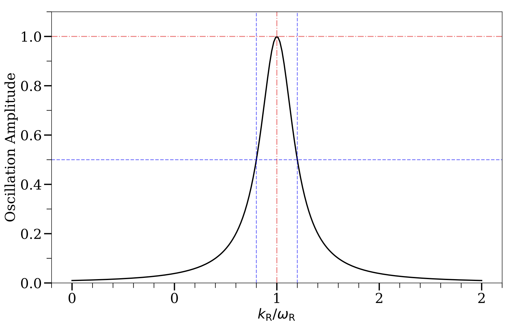
The resonance of Rabi oscillations occurs when $\vec{H}' _ 3=0$ in the corotating frame and $s_3$ oscillates between $+1/2$ (the low energy state) and $-1/2$ (the high energy state). The transition amplitude is determined by the relative detuning $\RD$ as illustrated by the two numerical examples in Fig. Rabi Oscillations. The resonance width is determined by the amplitude of the driving field $A_\RR$ as shown in Fig. Rabi Oscillations Width.
Rabi Oscillations
The transition probabilities $P$ between the energy states of a two-level quantum system when external driving fields with frequencies $k_\RR = \omega_\RR$ and $k_\RR=1.1\omega_\RR$ are applied, respectively. The corresponding relative detunings are $\RD = 0$ and $\RD = 1$, respectively. The amplitudes of the driving fields are $A_\RR=0.1\omega_\RR$ in both cases.
Rabi Oscillation Width
The amplitude of Rabi oscillations as a function of the frequency of the external driving field $k_\RR$. The maximum amplitude occurs at $k_\RR/\omega_\RR=1$. The resonance width is defined to be the difference of $k_\RR$ at which the amplitudes are 1/2.
In many cases, the two-level quantum system has more than one driving field. I will refer to each of the driving fields as a Rabi mode. Here I consider the Hamiltonian with two Rabi modes: $$ \begin{align} \mathsf H_{\mathrm R} =& -\frac{\omega_{\mathrm R}}{2}\sigma_3 - \frac{A_{1} }{2} \left( \cos(k_{1} t )\sigma_1 - \sin(k_{1} t ) \sigma_2\right) \nonumber\\ & - \frac{A_{2} }{2} \left( \cos(k_{2} t)\sigma_1 - \sin(k_{2} t ) \sigma_2\right). \label{chap:matter-sec:single-frequency-eqn:hamiltonian-two-level} \end{align} $$ I decompose it into $\vec{H}_ {\mathrm R}=\vec{H} _ 3 + \vec{H}_{1} + \vec{H}_2$, where $$ \begin{equation*} \vec{H}_1 = \begin{pmatrix} A_{1} \cos(k_{1}t) \\ -A_{1} \sin(k_{1}t) \\ 0 \end{pmatrix} \quad\text{and}\quad \vec{H}_2 = \begin{pmatrix} A_{2} \cos(k_{2}t) \\ -A_{2} \sin(k_{2}t) \\ 0 \end{pmatrix}. \end{equation*} $$ I will assume that the first Rabi mode $\vec{H}_1$ is almost on resonance, and the second one $\vec H_2$ is off resonance, i.e., $$ \begin{equation} \RD_1 \lesssim 1 \quad \text{and} \quad \RD_2 \gg 1, \end{equation} $$ where $$ \begin{equation} \RD_i\equiv \frac{\lvert k_i -\omega_{\mathrm R}\rvert}{\lvert A_i\rvert} \end{equation} $$ is the relative detuning of the $i$th Rabi mode.
Although the second Rabi mode is off resonance, it can interfere with the Rabi oscillation caused by the first Rabi mode. To see this effect, I will use the frame that corotates with $\vec H_2$. In the corotating frame, the two Rabi modes have frequencies $k_1'=k_1-k_2$ and $k_2'=0$, respectively, and $\vec H'_ 3 = ( 0,0, \omega_{\RR}- k_2 )^{\mathrm{T}}$. Obviously, the Hamiltonian vector in this corotating frame is similar to Eqn. \eqref{chap:matter-eqn:rabi-hamiltonian-h3-hplus} except with the replacements $$ \begin{equation} \vec H_3 \to \vec H'_3 + \vec H'_2 \quad \text{and} \quad \vec H_+ \to \vec H'_1. \end{equation} $$ I will further assume that $\lvert A_2\rvert \ll \omega_\RR$ so that the new energy gap is $$ \begin{align} \tilde\omega_{\mathrm{R}}' &\equiv \lvert \vec H'_3 + \vec H'_2 \rvert \Sign (\omega_\RR - k_2) \nonumber\\ &= \Sign (\omega_{\RR}- k_2 ) \sqrt{ (\omega_{\RR}- k_2 )^2 + A_2^2 } \nonumber\\ &\approx \omega_{\mathrm R} - k_2 + \frac{1}{2}\frac{A_2^2}{\omega_{\mathrm R} - k_2}, \label{eq-new-energy-gap-due-to-second-mode-approximation} \end{align} $$ where I have kept only up to the first order of the Taylor series. I can calculate the new relative detuning of the system to be $$ \begin{align} \RD' &= \frac{\lvert k_1' - \tilde \omega_{\mathrm R}' \rvert}{\lvert A_1 \rvert}\nonumber\\ &\approx \left \lvert \frac{ k_1-\omega_{\mathrm R}}{ A_1} + \frac{ A_2^2 }{2 A_1 ( k_2 - \omega_{\mathrm R})} \right \rvert. \label{app:chap:matter-eq:relative-detuning-changed} \end{align} $$ One can adjust the frequency of the off-resonance Rabi mode $k_2$ to decrease or increase $\RD$ so that the system is closer to or further away from the resonance. The criterion for the off-resonance Rabi mode to have a significant impact on the Rabi resonance is $$ \begin{equation} \left\lvert \frac{ A_2^2 }{2 A_1 ( k_2 - \omega_{\mathrm R})} \right\rvert \gtrsim 1 \quad \text{or} \quad \lvert A_2\rvert \gtrsim \sqrt{ 2 \lvert A_1 (k_2 - \omega_\RR) \rvert } \label{chap:matter-sec:single-frequency-eqn:criterion-for-a2} \end{equation} $$