Flavor Instabilities and Dispersion-Relation Gaps
One can find the flavor instabilities of a neutrino medium by solving the dispersion relations (DR) between $\omega$ and $\mathbf k$ from Eqn.~\eqref{eqn-dr-determinant-equation}. A negative imaginary component of $\omega$ indicates a flavor instability in time, and a positive imaginary component of $\mathbf k \cdot \hat{\mathbf z}$ indicates a flavor instability in the $+z$ direction. I. Izaguirre et al. conjectured that the flavor instabilities exist in the gaps between the real branches of the dispersion relations 1. In the first part this section I will first explain this conjecture, and in the second part I will show that this conjecture is actually incorrect.
Conjecture of the Relation between Flavor Instabilities and DR Gaps
I will consider a model with neutrinos emitted symmetrically about the $z$ axis. For this model, the characteristic equation \eqref{eqn-dr-determinant-equation} reduces to $$ \begin{align} &\det \left( \omega \mathsf{I} + \frac{1}{2} \begin{pmatrix} I_0 & 0 & 0 & -I_1 \\ 0 & -\frac{1}{2} (I_0 - I_2) & 0 & 0 \\ 0 & 0 & -\frac{1}{2} (I_0 - I_2) & 0 \\ I_1 & 0 & 0 & -I_2 \end{pmatrix}\right) =0, \label{eqn-det-polarization-tensor-axial} \end{align} $$ where $\mathsf I$ is the rank-4 identity matrix and $$ \begin{equation} I_m =\int_{-1}^{1} \dd u G(u) \frac{u^m}{1 - u/v_{\mathrm{ph}} }. \end{equation} $$ where $u=\cos\theta$, and $\vph=\omega/k$. Here I have assumed $\mathbf k = k \hat{\mathbf z}$. Eqn.~\eqref{eqn-det-polarization-tensor-axial} is satisfied if $$ \begin{equation} \omega = - \frac{1}{4} \left( I_0 - I_2 \pm \sqrt{ (I_0 + I_2 - 2 I_1) (I_0 + I_2 + 2 I_1) } \right) \label{eqn-mza} \end{equation} $$ or $$ \begin{equation} \omega = \frac{1}{4}(I_0 - I_2). \label{eqn-maa} \end{equation} $$ I will call the solutions to Eqn.~\eqref{eqn-mza} the symmetric solutions (SS$+$ and SS$-$ for the solutions to $\omega$ with the $+$ and $-$ signs) because they preserve the axial symmetry about the $z$ axis. I will call the solutions to Eqn.~\eqref{eqn-maa} the asymmetric solutions (AS) because they break the axial symmetry.
To illustrate the conjecture by I. Izaguirre et al., I will consider the two-angle model where the neutrinos are emitted with two zenith angles $\theta_1$ and $\theta_2$. The ELN of the two-angle model is $$ \begin{equation} G(u)= \mu \sum_{i=1,2} g_i \delta(u - u_i), \end{equation} $$ where $\mu = \sqrt{2}G_{\mathrm F} n$ is proportional to the neutrino number density $n$, $g_i$ are real numbers, and $u_i=\cos \theta_i$ ($i=1,2$). For any real $k$, the characteristic equations \eqref{eqn-mza} and \eqref{eqn-maa} are both quadratic equations of $\omega$ with two solutions In Fig. Dispersion Relations for Two-angel Model, I show the SS and AS of the dispersion relations $\omega(k)$ with $u_1=-0.6$, $u_2=0.6$ and $g_1=g_2=1$. In either case, both solutions $\omega(k)$ to the characteristic equations are real. However, there exist gaps between the DR curves where there is no real solution $k(\omega)$ for given real values of $\omega$. Because the characteristic equations are also quadratic equations of $k$ for any given real value of $\omega$, a pair of complex solutions $k (\omega) = k_{\mathrm R} (\omega) \pm \ri k_{\mathrm I}(\omega)$ exist in the DR gap of $\omega$ (see Fig. Dispersion Relations for Two-angel Model).
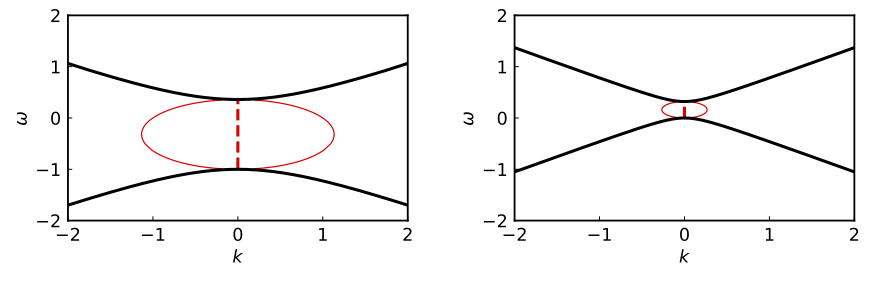
Dispersion Relations for Two-angel Model
The SS (left) and AS (right) of the dispersion relations for the two-angle model. The thick black curves represent $\omega(k)$ for real $k$. The red dashed and thin solid curves are $k_{\mathrm R}(\omega)$ and $k_{\mathrm R}(\omega) \pm k_{\mathrm I}(\omega)$ for real $\omega$ within the DR gap of $\omega$. Both $\omega$ and $k$ are measured in terms of the neutrino potential $\mu$.
The observation of the result of the two-angle model leads I. Izaguirre et al. to conjecture that the flavor instabilities are associated with the DR gaps. They also studied the dispersion relations using a continuous ELN distribution from a 1D supernova simulation 2 which are reproduced in Fig. Dispersion Relations for Garching Model.
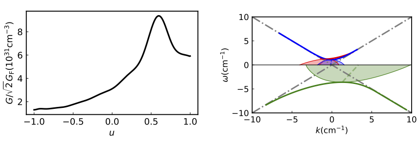
Dispersion Relations for Garching Model
The SS$+$ (green), SS$-$ (blue) and AS (red) of the dispersion relations (right panel) for a net electron flavor neutrino density distribution $n_{\nu_{\ee}}(u) -n_{\bar\nu_\ee}(u)$ obtained from a 1D supernova simulation by the Garching group (left panel). The thick solid curves represent the dispersion relations when both $\omega$ and $k$ are real. The dashed curves represent $k_{\mathrm R}(\omega)$ in the DR gap of $\omega$, and the thin solid curves (bounding the shaded regions) are $k_{\mathrm R}(\omega)\pm k_{\mathrm I}(\omega)$.
Refutation of the Conjecture
The association of the flavor instability in space, i.e., $k_{\mathrm I}(\omega)\neq 0$, with a DR gap in $\omega$ seems fortuitous for the two-angle model. As I explained previously, for the two-angle model, the characteristic equations are quadratic equation of $k$ for any given $\omega$. Therefore there always exists a pair of complex solutions between the DR gap in $\omega$. This is not the case when the neutrinos are emitted with more than two zenith angles.
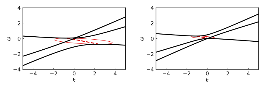
Dispersion Relations for Three-angel Model
The same as Fig. Dispersion Relations for Two-angel Model but for the three-angle model described in the text.
In Fig. Dispersion Relations for Three-angel Model, I show the dispersion relations of a three-angle model with ELN $$ \begin{align} G(u) = \frac{\mu}{2} \delta(u+0.1) + \mu \delta(u - 0.4) + \mu \delta(u-0.6). \end{align} $$ For this model, there exist complex solutions of $k(\omega)$ even though there is no DR gap in $\omega$. This is because the characteristic equations are cubic equations of $k$ for given $\omega$ which admit three solutions. In certain ranges of $\omega$ there is only one real solution of $k(\omega)$. The other two solutions must be complex which indicates flavor instabilities in space.
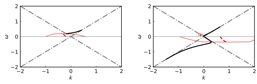
Dispersion Relations for Step-like ELN
The same as Fig. Dispersion Relations for Two-angel Model but for the ELN distribution in Eqn.~\eqref{chap:collective-sec:gap-eqn:eln-step-like}.
The conjecture between the flavor instabilities and DR gaps does not work for the models with a continuous ELN distribution $G(u)$ either. In Fig. Dispersion Relations for Step-like ELN, I show the dispersion relations for a step-like distribution $$ \begin{equation} G(u) = \begin{cases} -0.1 & \text{if } -1 < u < -0.3, \\ 1 & \text{otherwise.} \end{cases} \label{chap:collective-sec:gap-eqn:eln-step-like} \end{equation} $$ One sees that, for this model, the SS$+$ and SS$-$ solutions merge into a continuous DR curve so that there is no gap in $\omega$. However, there do exist complex solutions $k(\omega)$ for certain values of $\omega$.
As shown in Fig. Dispersion Relations for Garching Model and Fig. Dispersion Relations for Step-like ELN, AS dispersion relations $k(\omega)$ appear only in the region where $\omega > 0$. This can be proved analytically as follows. Suppose there exist dispersion relations $k(\omega) = k_{\mathrm R}(\omega) + \ri k_{\mathrm I}(\omega)$ for $\omega \to 0$. Using the Sokhotski–Plemelj theorem, I can rewrite the characteristic equation $$ \begin{equation} k = \frac{1}{4} \int \mathrm du G(u) \frac{ 1 - u^2 }{ \omega/k - u }. \label{chap:collective-eqn:k-omega-relation} \end{equation} $$ as $$ \begin{align} k_{\mathrm R} =& \frac{1}{4}\left( \mathcal{P} \int \mathrm d u G(u) \frac{ 1 - u^2 }{ - u } \right)\label{eqn-re-k-arbitrary-spectrum} \\ \lvert k_{\mathrm I} \rvert =& \frac{\pi}{4}G(0) \operatorname{Sign}\left( \omega \right), \label{eqn-k-arbitrary-spectrum} \end{align} $$ where $\mathcal P$ denotes the principal value of the integral. As long as $G(0)\neq 0$, $\omega$ must have the same sign as $G(0)$ which implies that $k(\omega)$ exists only on one side of the $\omega=0$ axis. For the two scenarios depicted in Fig. Dispersion Relations for Garching Model and Fig. Dispersion Relations for Step-like ELN, $G(0)>0$ and $k(\omega)$ exist only in the upper half plane of $\omega$. This shows that, at least near $\omega =0$, the absence of a DR $\omega(k)$, i.e., a “gap'' in $\omega$, is not always associated with the flavor instabilities in space.
Eqn.~\eqref{eqn-k-arbitrary-spectrum} can be used to determine the values of $k_{\mathrm R}$ and $k_{\mathrm I}$ in the limit of $\omega\to 0$ for the AS branch of the dispersion relations. One can apply the same method to the SS branches which gives $$ \begin{align} &\left(4 k_{\mathrm R} - J_{-1} + J_1 \right)^2 - \left( \operatorname{Sign}(\omega k_{\mathrm I} )\pi G(0) +4 k_{\mathrm I} \right)^2 \nonumber\\ =& - \left( J_{-1} + J_1 \right) \pi \operatorname{Sign}(\omega k_{\mathrm I} ) G(0) \label{chap:collective-eqn:dr-ss-general-limit-omega-0} \end{align} $$ and $$ \begin{equation} \lvert k_{\mathrm I} \rvert = - \frac{\pi}{4} G(0) \operatorname{Sign}(\omega ) \left( 1 \pm \frac{ J_{-1} + J_1 }{ 4 k_{\mathrm R} - J_{-1} + J_1} \right), \label{chap:collective-eqn:dr-ss-general-limit-omega-0-ya} \end{equation} $$ where $$ \begin{equation} J_{n} = \mathcal P \int G(u)u^n \mathrm du, \end{equation} $$ and the $+$ and $-$ signs are for SS$+$ and SS$-$, respectively. Eqn.~\eqref{chap:collective-eqn:dr-ss-general-limit-omega-0} and Eqn.~\eqref{chap:collective-eqn:dr-ss-general-limit-omega-0-ya} show that $k(\omega)$ exists on both sides of the $\omega=0$ axis but may be different for SS$+$ and SS$-$.
Ignacio Izaguirre, "Fast Pairwise Conversion of Supernova Neutrinos: A Dispersion Relation Approach", Physical Review Letters 118, 021101 (2017) . ↩︎
The data is from the Garching Core-Collapse Supernova Archive at http://wwwmpa.mpa-garching.mpg.de/ccsnarchive/archive.html ↩︎