Two-Beam Model and Flavor Instabilities
During the synchronized flavor transformation, the whole neutrino medium behaves as if there was a single neutrino oscillating with the mean frequency $\langle \omega_\vv \rangle$ in vacuum. Under certain conditions, the neutrino self-interaction potential can cause the neutrino medium to evolve in a way completely different than vacuum oscillations. I will illustrate this phenomenon using the two-beam neutrino model.
Two-Beam Line Model
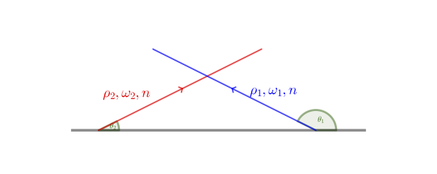
The geometry of two-beam model. The $i$th ($i=1,2$) neutrino beam has emission angle $\theta_i$, vacuum oscillation frequency $\omega_i$ and density matrix $\rho_i$. Both neutrino beams have the same number flux $n$.
In the two-beam model, neutrinos and antineutrinos are constantly emitted in two different directions from a plane which we assume to be the $x$-$y$ plane. I define the emission angles of the neutrino beams $\theta_1$ and $\theta_2$ to be inside the plane spanned by the velocity vectors of the two neutrino beams (see Fig. Two-Beam Line Model). I will assume that the neutrino emission plane is homogeneous and that the neutrino and antineutrino have the same density $n$ in the emission plane. I will also assume that the matter density vanishes everywhere in space.
The Hamiltonian of the $i$th neutrino beam in the vacuum basis is $$ \begin{align} \mathsf H_i &= -\frac{\omega_i}{2} \sigma_3 + \mu ( \rho_1 - \rho_2), \end{align} $$ where $\omega_1 = \eta\omega_\vv$ for the neutrino beam and $\omega_2=-\eta\omega_\vv$ for the antineutrino beam, $$ \begin{align} \mu = \sqrt{2} G_{\mathrm F} (1 - \cos(\theta_1 - \theta_2)) n \end{align} $$ is the neutrino self-interaction potential.
I will assume that the neutrino and antineutrino are emitted in the pure electron flavor at $z=0$. I will also assume the vacuum mixing angle $\theta_\vv \ll 1$. Therefore, the flavor density matrix of the $i$th neutrino beam in the vacuum basis at $z=0$ is $$ \begin{equation} \rho_i (z=0) \approx \begin{pmatrix} 1 & \epsilon_i (0) \\ \epsilon_i^* (0) & 0 \end{pmatrix}, \label{chap:collective-sec:two-beams-eqn:density-matrix-perturbed} \end{equation} $$ where $$ \begin{equation} \epsilon_i(0) = \sin (2\theta_\vv) \ll 1. \end{equation} $$
Numerical Solution to Two-beam Line Model
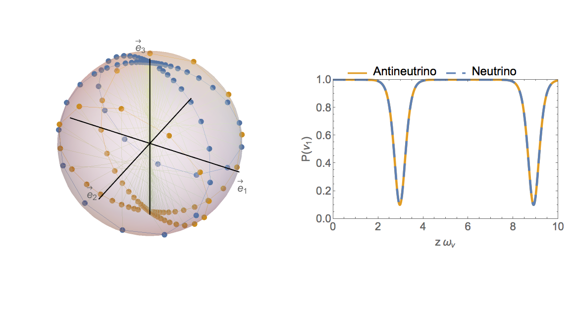
The numerical solution to the two-beam model. The left panel shows the position of the flavor isospins of the neutrino beam (in blue) and the antineutrino beam (in orange). The right panel shows the probabilities as functions of distance $z$ (in unit of $\omega_\vv^{-1}$) for the neutrino and antineutrino to remain in the $\ket{\nu_1}$ and $\ket{\bar\nu_1}$ states, which are the same as the survival probabilities of the electron flavor when the mixing angle $\theta_\vv \ll 1$. In this calculation, the emission angles are $\theta_1=5\pi/6$ and $\theta_2=\pi/6$, the neutrino self-interaction potential is $\mu=5 \omega_\vv$, and the neutrino mass hierarchy is inverted.
I solve the two-beam model numerically with $\epsilon_i = 10^{-3}$ and $\eta=-1$. The solution is shown in Fig. Numerical Solution to Two-beam Line Model. When $\omega_\vv z \ll 1$, the flavor isospin of the neutrino stays in the electron flavor state, i.e., in the direction of third axis $\vec e_3$ in the flavor space (see the left panel of Fig. Numerical Solution to Two-beam Line Model). Accordingly, the electron flavor survival probability $P_{\nu_\ee}\approx 1$ at small $z$ but falls down rapidly at a certain value of $z$ (see the right panel of Fig. Numerical Solution to Two-beam Line Model). Then both the flavor isospin and $P_{\nu_\ee}$ come back to their original positions until they fall down again. The flavor isospin of the antineutrino follows a similar pattern but is in a different direction. This flavor transformation phenomenon is clearly different from the vacuum oscillations shown in Fig. Two-Flavor Oscillations in Vacuum.
To gain a deeper understanding of the collective oscillation phenomenon, I will focus on the linear regime where $\lvert \epsilon_i(z) \rvert \ll 1$. The equation of motion is linearized in this regime and becomes $$ \begin{equation} \ri \partial_z \begin{pmatrix} \epsilon_1 \\ \epsilon_2 \end{pmatrix} = \begin{pmatrix} \mu + \eta\omega_\vv & - \mu \\ \mu & - \eta\omega_\vv - \mu \end{pmatrix} \begin{pmatrix} \epsilon_1 \\ \epsilon_2 \end{pmatrix}. \label{chap:collective-sec:bipolar-linearized-eom} \end{equation} $$ This equation has two normal modes which correspond to the collective modes of neutrino oscillations: $$ \begin{equation} \begin{pmatrix} \epsilon_1 (z) \\ \epsilon_2 (z) \end{pmatrix} = \begin{pmatrix} Q_{1\pm} \\ Q_{2\pm} \end{pmatrix} e^{i K_{z\pm} z}, \label{chap:collective-sec:two-beams-eqn:equation-of-motion-collective-mode-assumption} \end{equation} $$ where $(Q_{1\pm}, Q_{2\pm})^{\mathrm T}$ are the eigenvectors of the two normal modes, and $$ \begin{equation} K_{z\pm} = \pm \sqrt{ \omega_\vv (\omega_\vv + 2 \eta \mu) } \end{equation} $$ are the wavenumbers of the corresponding modes. For the normal mass hierarchy, $\eta = 1$, and $K_{z\pm}$ are always real. In this case, the electron flavor probability $P_{\nu_\ee}$ is always approximately 1. However, for the inverted neutrino mass hierarchy, $\eta=-1$, and $K_{z\pm}$ are imaginary when $\mu > \omega_\vv/2$. The normal mode with wavenumber $K_{z-} = -\ri \sqrt{ \omega_\vv (2 \mu-\omega_\vv) }$ is a runaway solution which explains the rapid decrease of $P_{\nu_\ee}$ in Fig. Numerical Solution to Two-beam Line Model.